200 lines of python code to demonstrate DQN with Keras

Overview

This project demonstrates how to use the Deep-Q Learning algorithm with Keras together to play FlappyBird.

This article is intended to target newcomers who are interested in Reinforcement Learning.

Installation Dependencies:

(Update : 13 March 2017, code and weight file has been updated to support latest version of tensorflow and keras)

Python 2.7
Keras 1.0
pygame
scikit-image

How to Run?

CPU only/TensorFlow

git clone https://github.com/yanpanlau/Keras-FlappyBird.git
cd Keras-FlappyBird
python qlearn.py -m "Run"

GPU version (Theano)

git clone https://github.com/yanpanlau/Keras-FlappyBird.git
cd Keras-FlappyBird
THEANO_FLAGS=device=gpu,floatX=float32,lib.cnmem=0.2 python qlearn.py -m "Run"

lib.cnmem=0.2 means you assign only 20% of the GPU’s memory to the program.

If you want to train the network from beginning, delete “model.h5” and run qlearn.py -m “Train”

What is Deep Q-Network?

Deep Q-Network is a learning algorithm developed by Google DeepMind to play Atari games. They demonstrated how a computer learned to play Atari 2600 video games by observing just the screen pixels and receiving a reward when the game score increased. The result was remarkable because it demonstrates the algorithm is generic enough to play various games.

The following post is a must-read for those who are interested in deep reinforcement learning.

Demystifying Deep Reinforcement Learning

Code Explanation (in details)

Let’s go though the example in qlearn.py, line by line. If you familiar with Keras and DQN, you can skip this session

The code simply does the following:

The code receives the Game Screen Input in the form of a pixel array
The code does some image pre-processing
The processed image will be fed into a neural network (Convolution Neural Network), and the network will then decide the best action to execute (Flap or Not Flap)
The network will be trained millions of times, via an algorithm called Q-learning, to maximize the future expected reward.

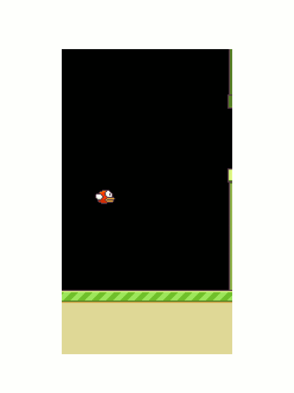
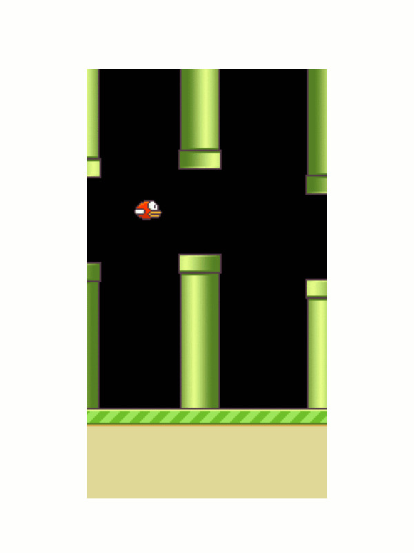
Game Screen Input

First of all, the FlappyBird is already written in Python via pygame, so here is the code snippet to access the FlappyBird API

import wrapped_flappy_bird as game
x_t1_colored, r_t, terminal = game_state.frame_step(a_t)

The idea is quite simple, the input is a_t (0 represent don’t flap, 1 represent flap), the API will give you the next frame x_t1_colored, the reward (0.1 if alive, +1 if pass the pipe, -1 if die) and terminal is a boolean flag indicates whether the game is FINISHED or NOT. We also followed DeepMind suggestion to clip the reward between [-1,+1] to improve the stability. I have not yet get a chance to test out different reward functions but it would be an interesting exercise to see how the performance is changed with different reward functions.

Interesting readers can modify the reward function in game/wrapped_flappy_bird.py”, under the function **def frame_step(self, input_actions)

Image pre-processing

In order to make the code train faster, it is vital to do some image processing. Here are the key elements:

I first convert the color image into grayscale
I crop down the image size into 80x80 pixel
I stack 4 frames together before I feed into neural network.

Why do I need to stack 4 frames together? This is one way for the model to be able to infer the velocity information of the bird.

x_t1 = skimage.color.rgb2gray(x_t1_colored)
x_t1 = skimage.transform.resize(x_t1,(80,80))
x_t1 = skimage.exposure.rescale_intensity(x_t1, out_range=(0, 255))

x_t1 = x_t1.reshape(1, 1, x_t1.shape[0], x_t1.shape[1])
s_t1 = np.append(x_t1, s_t[:, :3, :, :], axis=1)

x_t1 is a single frame with shape (1x1x80x80) and s_t1 is the stacked frame with shape (1x4x80x80). You might ask, why the input dimension is (1x4x80x80) but not (4x80x80)? Well, it is a requirement in Keras so let’s stick with it.

Note: Some readers may ask what is axis=1? It means that when I stack the frames, I want to stack on the “2nd” dimension. i.e. I am stacking under (1x4x80x80), the 2nd index.

Convolution Neural Network

Now, we can input the pre-processed screen into the neural network, which is a convolution neural network:

def buildmodel():
    print("Now we build the model")
    model = Sequential()
    model.add(Convolution2D(32, 8, 8, subsample=(4,4),init=lambda shape, name: normal(shape, scale=0.01, name=name), border_mode='same',input_shape=(img_channels,img_rows,img_cols)))
    model.add(Activation('relu'))
    model.add(Convolution2D(64, 4, 4, subsample=(2,2),init=lambda shape, name: normal(shape, scale=0.01, name=name), border_mode='same'))
    model.add(Activation('relu'))
    model.add(Convolution2D(64, 3, 3, subsample=(1,1),init=lambda shape, name: normal(shape, scale=0.01, name=name), border_mode='same'))
    model.add(Activation('relu'))
    model.add(Flatten())
    model.add(Dense(512, init=lambda shape, name: normal(shape, scale=0.01, name=name)))
    model.add(Activation('relu'))
    model.add(Dense(2,init=lambda shape, name: normal(shape, scale=0.01, name=name)))
   
    adam = Adam(lr=1e-6)
    model.compile(loss='mse',optimizer=adam)
    print("We finish building the model")
    return model

The exact architecture is following : The input to the neural network consists of an 4x80x80 images. The first hidden layer convolves 32 filters of 8 x 8 with stride 4 and applies ReLU activation function. The 2nd layer convolves a 64 filters of 4 x 4 with stride 2 and applies ReLU activation function. The 3rd layer convolves a 64 filters of 3 x 3 with stride 1 and applies ReLU activation function. The final hidden layer is fully-connected consisted of 512 rectifier units. The output layer is a fully-connected linear layer with a single output for each valid action.

So wait, what is convolution? The easiest way to understand a convolution is by thinking of it as a sliding window function apply to a matrix. The following gif file should help to understand.

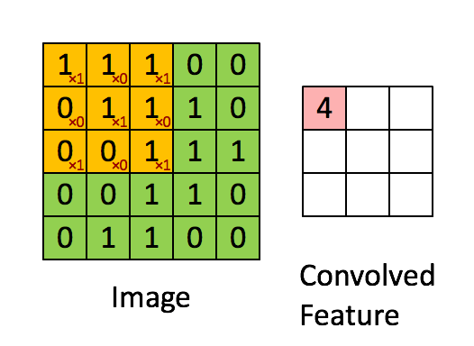
Convolution with 3×3 Filter. Source: http://deeplearning.stanford.edu/wiki/index.php/Feature_extraction_using_convolution

You might ask what’s the purpose the convolution? It actually help computer to learn higher features like edges and shapes. The example below shows how the edges are stand out after a convolution filter is applied

Using Convolution to detect Edges

For more details about Convolution in Neural Network, please read Understanding Convolution Neural Networks for NLP

Note

Keras makes it very easy to build convolution neural network. However, there are few things I would like to highlight

A) It is important to choose a right initialization method. I choose normal distribution with $\sigma=0.01$

init=lambda shape, name: normal(shape, scale=0.01, name=name)

B) The ordering of the dimension is important, the default setting is 4x80x80 (Theano setting), so if your input is 80x80x4 (Tensorflow setting) then you are in trouble because the dimension is wrong. Alert: If your input dimension is 80x80x4 (Tensorflow setting) you need to set dim_ordering = tf (tf means tensorflow, th means theano)

C) In Keras, subsample=(2,2) means you down sample the image size from (80x80) to (40x40). In ML literature it is often called “stride”

D) We have used an adaptive learning algorithm called ADAM to do the optimization. The learning rate is 1-e6.

Interested readers who want to learn more various learning algoithms please read below

An overview of gradient descent optimization algorithms

DQN

Finally, we can using the Q-learning algorithm to train the neural network.

So, what is Q-learning? In Q-learning the most important thing is the Q-function : Q(s, a) representing the maximum discounted future reward when we perform action a in state s. Q(s, a) gives you an estimation of how good to choose an action a in state s.

REPEAT : Q(s, a) representing the maximum discounted future reward when we perform action a in state s

You might ask 1) Why Q-function is useful? 2) How can I get the Q-function?

Let me give you an analogy of the Q-function: Suppose you are playing a difficult RPG game and you don’t know how to play it well. If you have bought a strategy guide, which is an instruction book that contain hints or complete solutions to a specific video game, then playing that video game is easy. You just follow the guidiance from the strategy book. Here, Q-function is similar to a strategy guide. Suppose you are in state s and you need to decide whether you take action a or b. If you have this magical Q-function, the answers become really simple – pick the action with highest Q-value!

$\pi(s) = {argmax}_{a} Q(s,a)$

Here, $\pi$ represents the policy, which you will often see in the ML literature.

How do we get the Q-function? That’s where Q-learning is coming from. Let me quickly derive here:

Define total future reward from time t onward

$R_t = r_t + r_{t+1} + r_{t+2} ... + r_n$

But because our environment is stochastic, we can never be sure, the more future we go, the more uncertain. Therefore, it is common to use discount future reward instead

$R_t = r_t + \gamma r_{t+1} + \gamma^{2} r_{t+2} ... + \gamma^{n-t} r_n$

which, can be written as

$R_t = r_t + \gamma * R_{t+1}$

Recall the definition of Q-function (maximum discounted future reward if we choose action a in state s)

$Q(s_t, a_t) = max R_{t+1}$

therefore, we can rewrite the Q-function as below

$Q(s, a) = r + \gamma * max_{a^{'}} Q(s^{'}, a^{'})$

In plain English, it means maximum future reward for this state and action (s,a) is the immediate reward r plus maximum future reward for the next state $s^{'}$ , action $a^{'}$

We could now use an iterative method to solve for the Q-function. Given a transition $(s, a, r, s^{'})$ , we are going to convert this episode into training set for the network. i.e. We want $r + \gamma max_a Q (s,a)$ to be equal to $Q(s,a)$ . You can think of finding a Q-value is a regession task now, I have a estimator $r + \gamma max_a Q (s,a)$ and a predictor $Q(s,a)$ , I can define the mean squared error (MSE), or the loss function, as below:

Define a loss function

$L = [r + \gamma max_{a^{'}} Q (s^{'},a^{'}) - Q(s,a)]^{2}$

Given a transition $(s, a, r, s^{'})$ , how can I optimize my Q-function such that it returns the smallest mean squared error loss? If L getting smaller, we know the Q-function is getting converged into the optimal value, which is our “strategy book”.

Now, you might ask, where is the role of the neural network? This is where the DEEP Q-Learning comes in. You recall that $Q(s,a)$ , is a stategy book, which contains millions or trillions of states and actions if you display as a table. The idea of the DQN is that I use the neural network to COMPRESS this Q-table, using some parameters $\theta$ (We called it weight in Neural Network). So instead of handling a large table, I just need to worry the weights of the neural network. By smartly tuning the weight parameters, I can find the optimal Q-function via the various Neural Network training algorithm.

$Q(s,a) = f_{\theta}(s)$

where $f$ is our neural network with input $s$ and weight parameters $\theta$

Here is the code below to demonstrate how it works

if t > OBSERVE:
    #sample a minibatch to train on
    minibatch = random.sample(D, BATCH)

    inputs = np.zeros((BATCH, s_t.shape[1], s_t.shape[2], s_t.shape[3]))   #32, 80, 80, 4
    targets = np.zeros((inputs.shape[0], ACTIONS))                         #32, 2

    #Now we do the experience replay
    for i in range(0, len(minibatch)):
        state_t = minibatch[i][0]
        action_t = minibatch[i][1]   #This is action index
        reward_t = minibatch[i][2]
        state_t1 = minibatch[i][3]
        terminal = minibatch[i][4]
        # if terminated, only equals reward

        inputs[i:i + 1] = state_t    #I saved down s_t

        targets[i] = model.predict(state_t)  # Hitting each buttom probability
        Q_sa = model.predict(state_t1)

        if terminal:
            targets[i, action_t] = reward_t
        else:
            targets[i, action_t] = reward_t + GAMMA * np.max(Q_sa)

        loss += model.train_on_batch(inputs, targets)

    s_t = s_t1
    t = t + 1

Experience Replay

If you examine the code above, there is a comment called “Experience Replay”. Let me explain what it does: It was found that approximation of Q-value using non-linear functions like neural network is not very stable. The most important trick to solve this problem is called experience replay. During the gameplay all the episode $(s, a, r, s^{'})$ are stored in replay memory D. (I use Python function deque() to store it). When training the network, random mini-batches from the replay memory are used instead of most the recent transition, which will greatly improve the stability.

Exploration vs. Exploitation

There is another issue in the reinforcement learning algorithm which called Exploration vs. Exploitation. How much of an agent’s time should be spent exploiting its existing known-good policy, and how much time should be focused on exploring new, possibility better, actions? We often encounter similar situations in real life too. For example, we face on which restaurant to go to on Saturday night. We all have a set of restaurants that we prefer, based on our policy/strategy book $Q(s,a)$ . If we stick to our normal preference, there is a strong probability that we’ll pick a good restaurant. However, sometimes, we occasionally like to try new restaurants to see if they are better. The RL agents face the same problem. In order to maximize future reward, they need to balance the amount of time that they follow their current policy (this is called being “greedy”), and the time they spend exploring new possibilities that might be better. A popular approach is called $\epsilon$ greedy approach. Under this approach, the policy tells the agent to try a random action some percentage of the time, as defined by the variable $\epsilon$ (epsilon), which is a number between 0 and 1. The strategy will help the RL agent to occasionally try something new and see if we can achieve ultimate strategy.

if random.random() <= epsilon:
    print("----------Random Action----------")
    action_index = random.randrange(ACTIONS)
    a_t[action_index] = 1
        else:
    q = model.predict(s_t)       #input a stack of 4 images, get the prediction
    max_Q = np.argmax(q)
    action_index = max_Q
    a_t[max_Q] = 1

I think that’s it. I hope this blog will help you to understand how DQN works.

FAQ

My training is very slow

You might need a GPU to accelerate the calculation. I used a TITAN X and train for at least 1 million frames to make it work

Future works and thoughts

Current DQN depends on large experience replay. Is it possible to replace it or even remove it?
How can one decide on the optimal Convolution Neural Network?
Training is very slow, how to speed it up/to make the model converge faster?
What does the Neural Network actually learn? Is the knowledge transferable?

I believe the questions are still not resolved and it’s an active research area in Machine Learning.

Reference

[1] Mnih Volodymyr, Koray Kavukcuoglu, David Silver, Andrei A. Rusu, Joel Veness, Marc G. Bellemare, Alex Graves, Martin Riedmiller, Andreas K. Fidjeland, Georg Ostrovski, Stig Petersen, Charles Beattie, Amir Sadik, Ioannis Antonoglou, Helen King, Dharshan Kumaran, Daan Wierstra, Shane Legg, and Demis Hassabis. Human-level Control through Deep Reinforcement Learning. Nature, 529-33, 2015.

Disclaimer

This work is highly based on the following repos:

https://github.com/yenchenlin/DeepLearningFlappyBird

http://edersantana.github.io/articles/keras_rl/

Acknowledgement

I must thank to @hardmaru to encourage me to write this blog. I also thank to @fchollet to help me on the weight initialization in Keras and @edersantana his post on Keras and reinforcement learning which really help me to understand it.

Ben Lau

Using Keras and Deep Q-Network to Play FlappyBird