300 lines of python code to demonstrate DDPG with Keras
Overview
This is the second blog posts on the reinforcement learning. In this project we will demonstrate how to use the Deep Deterministic Policy Gradient algorithm (DDPG) with Keras together to play TORCS (The Open Racing Car Simulator), a very interesting AI racing game and research platform.
Installation Dependencies:
- Python 2.7
- Keras 1.1.0
- Tensorflow r0.10
- gym_torcs
How to Run?
git clone https://github.com/yanpanlau/DDPG-Keras-Torcs.git
cd DDPG-Keras-Torcs
cp *.* ~/gym_torcs
cd ~/gym_torcs
python ddpg.py
(Change the flag train_indicator=1 in ddpg.py if you want to train the network)
Motivation
As a typical child growing up in Hong Kong, I do like watching cartoon movies. One of my favorite movies is called GPX Cyber Formula. It is an anime series about Formula racing in the future, a time when the race cars are equipped with super-intelligent AI computer system called “Cyber Systems”. The AI can communicate with humans interactively and it can assist drivers to race in various extreme situations. Although we are still far away from building super-intelligent AI system, the latest development in the computer vision and deep learning has created an exciting era for me to fulfill my little dream – to create a cyber system called “Asurada”.

Why TORCS
I think it is important to study TORCS because:
- It looks cool, it’s really cool to see the AI can learn how to drive
- You can visualize how the neural network learns over time and inspect its learning process, rather than just looking at the final result
- It is easy to visualize when the neural network stuck in local minimun
- It can help us understand machine learning technique in automated driving, which is important for self-driving car technologies
Background
In the previous blog post Using Keras and Deep Q-Network to Play FlappyBird we demonstrate using Deep Q-Network to play FlappyBird. However, a big limitation of Deep Q-Network is that the outputs/actions are discrete while the action like steering are continuous in car racing. An obvious approach to adapt DQN to continuous domains is to simply discretize the action space. However, we encounter the “curse of dimensionality” problem. For example, if you discretize the steering wheel from -90 to +90 degrees in 5 degrees each and acceleration from 0km to 300km in 5km each, your output combinations will be 36 steering states times 60 velocity states which equals to 2160 possible combinations. The situation will be worse when you want to build robots to perform something very specialized, such as brain surgery that requires fine control of actions and naive discretization will not able to achieve the required precision to do the operations.
Google Deepmind has devised a new algorithm to tackle the continuous action space problem by combining 3 techniques together 1) Deterministic Policy-Gradient Algorithms 2) Actor-Critic Methods 3) Deep Q-Network called Deep Deterministic Policy Gradients (DDPG)
The original paper in 1) is not easy for non-machine learning expert to digest so I will sketch the proof here. If you are already familiar with the algorithm you can directly go to Keras code session.
Policy Network
First, we are going to define a policy network that implements our AI-driver. This network will take the state of the game (for example, the velocity of the car, the distance between the car and the track axis etc) and decide what we should do (steer left or right, hit the gas pedal or hit the brake). It is called Policy-Based Reinforcement Learning because we will directly parametrize the policy
here, s is the state , a is the action and is the model parameters of the policy network. We can think of policy is the agent’s behaviour, i.e. a function to map from state to action.
Deterministic vs Stochastic Policy
Please note that there are 2 types of the policies:
Deterministic policy:
Stochastic policy:
Why do we need stochastic policies in addition to a deterministic policy? It is easy to understand a deterministic policy. I see a particular state input, then I take a particular action. But sometimes deterministic policy won’t work, like in the example of GO, where your first state is the empty board like below:
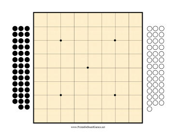
If you use same deterministic strategy, your network will always place the stone in a “particular” position which is a highly undesirable behaviour since it makes you predictable by your opponent. In that situation, a stochastic policy is more suitable than deterministic policy.
Policy Objective Functions
So how can I find ? Actually, we can use the reinforcement technique to solve it. For example, suppose the AI is trying to learn how to make a left turn. At the beginning the AI may simply not steer the wheel and hit the curb and receive a negative reward, so the neural network will adjust the model parameters such that next time it will try to avoid hitting the curb. After many attempts it will have discovered that “argh if I turn the wheel a bit more to the left I won’t hit the curb so early”. In mathematics language, we call these policy objective functions.
Let’s define total discount future reward
An intuitive policy objective function will be the expectation of the total discount reward
or
where the expectations of the total reward R is calculated under some probability distribution parameterized by some
If you recall our previous blog that we have introduced the Q-function, which is maximum discounted future reward if we choose action a in state s
now in the continuous case we can use the SARSA formula
therefore, we can write the gradient of a deterministic policy as
Now, let’s apply the chain rule:
Silver el at. (2014) proved that this is the policy gradient, i.e. you will get the maximum expected reward as long as you update your model parameters following the gradient formula above.
Actor-Critic Algorithm
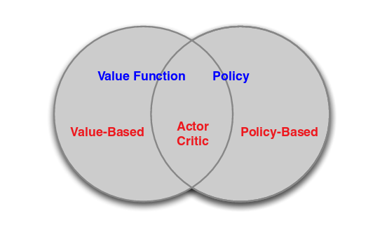
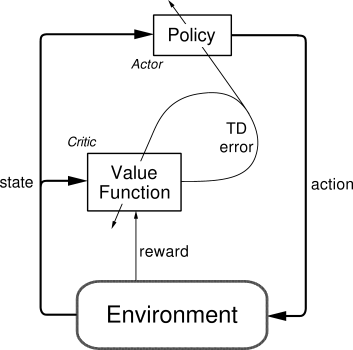
The Actor-Critic Algorithm is essentially a hybrid method to combine the policy gradient method and the value function method together. The policy function is known as the actor, while the value function is referred to as the critic. Essentially, the actor produces the action given the current state of the environment , while the critic produces a signal to criticizes the actions made by the actor. I think it is quite natural in the human’s world where the junior employee (actor) do the actual work and your boss (critic) criticizes your work and hopefully the junior employee can do it better next time. In our TORCS example, we use the continuous Q-learning (SARSA) as our critic model and use policy gradient method as our actor model. The following figure explains the relationships between Value Function/Policy Function and Actor-Critic Algorithm.
Going back to the previous equations, we can use the trick of the Deep-Q Network where we replace the Q-function as a neural network , where w is the weight of the neural network. Therefore, we arrived the Deep Deterministic Policy Gradient Formula:
where the policy parameters can be updated via stochastic gradient ascent.
Follow the previous DQN blog post, we could use an iterative method to solve for the Q-function, where we can setup the Loss function
the Q-value can be used to estimate the values of the current actor policy.
The following figure shows the actor-critic architecture from Sutton’s Book [2]
Keras Code Explanation
Actor Network
Let’s first talk about how to build the Actor Network in Keras. Here we used 2 hidden layers with 300 and 600 hidden units respectively. The output consist of 3 continuous actions, Steering, which is a single unit with tanh activation function (where -1 means max right turn and +1 means max left turn). Acceleration, which is a single unit with sigmoid activation function (where 0 means no gas, 1 means full gas). Brake, another single unit with sigmoid activation function (where 0 means no brake, 1 bull brake)
    def create_actor_network(self, state_size,action_dim):
        print("Now we build the model")
        S = Input(shape=[state_size])
        h0 = Dense(HIDDEN1_UNITS, activation='relu')(S)
        h1 = Dense(HIDDEN2_UNITS, activation='relu')(h0)
        Steering = Dense(1,activation='tanh',init=lambda shape, name: normal(shape, scale=1e-4, name=name))(h1)
        Acceleration = Dense(1,activation='sigmoid',init=lambda shape, name: normal(shape, scale=1e-4, name=name))(h1)
        Brake = Dense(1,activation='sigmoid',init=lambda shape, name: normal(shape, scale=1e-4, name=name))(h1)
        V = merge([Steering,Acceleration,Brake],mode='concat')
        model = Model(input=S,output=V)
        print("We finished building the model")
        return model, model.trainable_weights, S
We have used Keras function called Merge to combine 3 outputs together. Smart readers may ask why not using traditional Dense function like this
V = Dense(3,activation='tanh')(h1) There is a reason for that. First using 3 different Dense() function allows each continuous action have different activation function, for example, using tanh() for acceleration doesn’t make sense as tanh are in the range [-1,1] while the acceleration is in the range [0,1]
Please also noted that in the final layer we used the normal initialization with = 0 , = 1e-4 to ensure the initial outputs for the policy were near zero.
Critic Network
The construction of the Critic Network is very similar to the Deep-Q Network in the previous post. The only difference is that we used 2 hidden layers with 300 and 600 hidden units. Also, the critic network takes both the states and the action as inputs. According to the DDPG paper, the actions were not included until the 2nd hidden layer of Q-network. Here we used the Keras function Merge to merge the action and the hidden layer together
    def create_critic_network(self, state_size,action_dim):
        print("Now we build the model")
        S = Input(shape=[state_size])
        A = Input(shape=[action_dim],name='action2')
        w1 = Dense(HIDDEN1_UNITS, activation='relu')(S)
        a1 = Dense(HIDDEN2_UNITS, activation='linear')(A)
        h1 = Dense(HIDDEN2_UNITS, activation='linear')(w1)
        h2 = merge([h1,a1],mode='sum')
        h3 = Dense(HIDDEN2_UNITS, activation='relu')(h2)
        V = Dense(action_dim,activation='linear')(h3)
        model = Model(input=[S,A],output=V)
        adam = Adam(lr=self.LEARNING_RATE)
        model.compile(loss='mse', optimizer=adam)
        print("We finished building the model")
        return model, A, S
Target Network
It is a well-known fact that directly implementing Q-learning with neural networks proved to be unstable in many environments including TORCS. Deepmind team came up the solution to the problem is to use a target network, where we created a copy of the actor and critic networks respectively, that are used for calculating the target values. The weights of these target networks are then updated by having them slowly track the learned networks:
where . This means that the target values are constrained to change slowly, greatly improving the stability of learning.
It is extremely easy to implement target networks in Keras:
    def target_train(self):
        actor_weights = self.model.get_weights()
        actor_target_weights = self.target_model.get_weights()
        for i in xrange(len(actor_weights)):
            actor_target_weights[i] = self.TAU * actor_weights[i] + (1 - self.TAU)* actor_target_weights[i]
        self.target_model.set_weights(actor_target_weights)
Main Code
After we finished the network setup, Let’s go through the example in ddpg.py, our main code
The code simply does the following:
- The code receives the sensor input in the form of array
- The sensor input will be fed into our Neural Network, and the network will output 3 real numbers (value of the steering, acceleration and brake)
- The network will be trained many times, via the Deep Deterministic Policy Gradient, to maximize the future expected reward.
Sensor Input
In the TORCS there are 18 different types of sensor input, the details can be found here Simulated Car Racing Championship : Competition Software Manual. So which sensor input should we use? After some trial-and-error, I found the following inputs are useful:
| Name | Range (units) | Description |
|---|---|---|
| ob.angle | [-,+] | Angle between the car direction and the direction of the track axis |
| ob.track | (0, 200)(meters) | Vector of 19 range finder sensors: each sensor returns the distance between the track edge and the car within a range of 200 meters |
| ob.trackPos | (-,+) | Distance between the car and the track axis. The value is normalized w.r.t. to the track width: it is 0 when the car is on the axis, values greater than 1 or -1 means the car is outside of the track. |
| ob.speedX | (-,+)(km/h) | Speed of the car along the longitudinal axis of the car (good velocity) |
| ob.speedY | (-,+)(km/h) | Speed of the car along the transverse axis of the car |
| ob.speedZ | (-,+)(km/h) | Speed of the car along the Z-axis of the car |
| ob.wheelSpinVel | (0,+)(rad/s) | Vector of 4 sensors representing the rotation speed of wheels |
| ob.rpm | (0,+)(rpm) | Number of rotation per minute of the car engine |
Please note that we have normalized some of those value before feed into the neural network and some sensor inputs are not exposed in gym_torcs. The Advanced user needs to amend gym_torcs.py to change the parameters. [checkout the function make_observaton()]
Policy Selection
Now we can use the inputs above to feed into the neural network. The code is actually very simple:
    for j in range(max_steps):
        a_t = actor.model.predict(s_t.reshape(1, s_t.shape[0]))
        ob, r_t, done, info = env.step(a_t[0])
However, we immediately run into the two issues. First, how do we decide the reward? Second, how do we do exploration in the continuous action space?
Design of the rewards
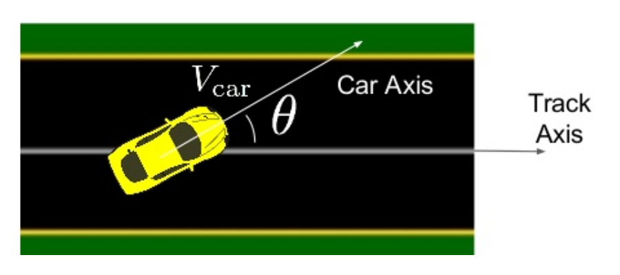
In the original paper, they used the reward function which is equal to the velocity of the car projected along the track direction as illustrated below:
However, I found that the training is not very stable as reported in the original paper.
On both low-dimensional and form pixels, some replicas were able to learn reasonable policies that are able to complete a circuit around the track though other replicas failed to learn a sensible policy
I believe the reason is that in the original policy the AI will try to accelerate the gas pedal very hard (to get maximum reward) and it hits the edge and the episode terminated very quickly. Therefore, the neural network stuck in a very poor local minimum. The new proposed reward function is below:
In plain English, we want to maximum longitudinal velocity (first term), minimize transverse velocity (second term), and we also penalize the AI if it constantly drives very off center of the track (third term)
I found the new reward function greatly improves the stability and the learning time of TORCS.
Design of the exploration algorithm
Another issue is how to design a right exploration algorithm in the continuous domain. In the previous blog post, we used greedy policy where the agent to try a random action some percentage of the time. However, this approach does not work very well in TORCS because we have 3 actions [steering,acceleration,brake]. If I just randomly choose the action from uniform random distribution we will generate some boring combinations [eg: the value of the brake is greater than the value of acceleration and the car simply not moving). Therefore, we add the noise using Ornstein-Uhlenbeck process to do the exploration.
Ornstein-Uhlenbeck process
What is Ornstein-Uhlenbeck process? In simple English it is simply a stochastic process which has mean-reverting properties.
here, means the how “fast” the variable reverts towards to the mean. represents the equilibrium or mean value. is the degree of volatility of the process. Interestingly, Ornstein-Uhlenbeck process is a very common approach to model interest rate, FX and commodity prices stochastically. (And a very common interview questions in finance quant interview). The following table shows the suggested values that I used in the code.
| Action | |||
|---|---|---|---|
| steering | 0.6 | 0.0 | 0.30 |
| acceleration | 1.0 | [0.3-0.6] | 0.10 |
| brake | 1.0 | -0.1 | 0.05 |
Basically, the most important parameters are the of the acceleration, where you want the car have some initial velocity and don’t stuck in a local minimum where the car keep pressing the brake and never hit the gas pedal. Readers feel free to change the parameters and see how the AI performs in various combinations. The code of the Ornstein-Uhlenbeck process is saved under OU.py
My finding is that the AI can learn a reasonable policy on the simple track if using a sensible exploration policy and revised reward function, like within ~200 episode.
Experience Replay
Similar to the FlappyBird case, we also used the Experience Replay to saved down all the episode in a replay memory. When training the network, random mini-batches from the replay memory are used instead of most the recent transition, which will greatly improve the stability. The following code snippet shows how it is done.
        buff.add(s_t, a_t[0], r_t, s_t1, done)
        # sample a random minibatch of N transitions (si, ai, ri, si+1) from replay buffer
        batch = buff.getBatch(BATCH_SIZE)
        states = np.asarray([e[0] for e in batch])
        actions = np.asarray([e[1] for e in batch])
        rewards = np.asarray([e[2] for e in batch])
        new_states = np.asarray([e[3] for e in batch])
        dones = np.asarray([e[4] for e in batch])
        y_t = np.asarray([e[1] for e in batch])

        target_q_values = critic.target_model.predict([new_states, actor.target_model.predict(new_states)])    #Still using tf

        for k in range(len(batch)):
            if dones[k]:
                y_t[k] = rewards[k]
            else:
                y_t[k] = rewards[k] + GAMMA*target_q_values[k]
Please note that when we calculated the target_q_values we do use the output of target-Network instead of the model instead. The used of the slow-varying target-Network will reduce the oscillations of the Q-value estimation, which greatly improve the stability of the learning.
Training
The actual training of the neural network is very simple, only contains 6 lines of code:
        loss += critic.model.train_on_batch([states,actions], y_t)
        a_for_grad = actor.model.predict(states)
        grads = critic.gradients(states, a_for_grad)
        actor.train(states, grads)
        actor.target_train()
        critic.target_train()
In plain English, we first update the critic by minimizing the loss
Then the actor policy is updated using the sampled policy gradient
recall is the deterministic policy:
therefore, it can be written as
The last 2 lines of the code update the target network
Results
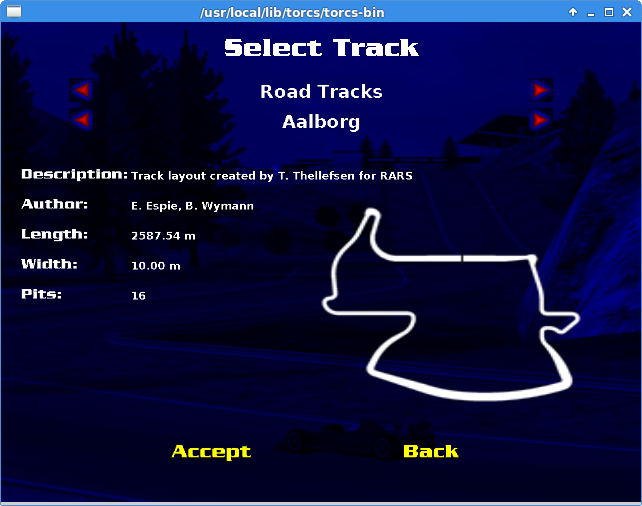
In order to test the policy, I choose a slightly difficult track called Aalborg as my training dataset. The figure below shows the layout of the track:
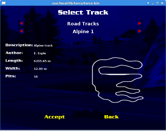
I trained the neural network with 2000 episodes and allowed Ornstein-Uhlenbeck process decay linearly in 100000 frames. (i.e. no more exploitation is applied after 100000 frames). I also validate my neural network by allowing the agent to drive on a much longer track called Alpine 1 (3 times longer). It is important to test the AI agents in other tracks to make sure the AI do not simply “memorize the track”, aka overfitting.
The first video shows the result of the Aalborg track, our training dataset.
I used the software avconv to capture my video output. (My computer is a bit slow therefore the Audio output is not very smooth). As you can see the agent learned a decent policy. (I took the video after the agent finished 2 loops)
The second video shows the result of the Alpine 1 track, our validation dataset.
The agent managed to drive for 3 minutes before the car spin and stop there.
Since the AI agent can drive on Alpine 1 track which is much longer than Aalborg track, we can say that the Neural Network did not overfit on the testing dataset. However, you can see the policy is still not optimal yet as the agent didn’t use the brake much.
Learn how to brake
It turns out that asking AI to learn how to brake is much harder than steering or acceleration. The reason is that the velocity of the car slow down when the brake is applied, therefore, the reward function is reduced and the AI agent is not keen to hit the brake at all. Also, if I allow the AI to hit the brake and the acceleration at the same time during the exploration phase, the AI will often hit the brake hard therefore we are stuck in very poor local minimum (as the car is not moving and no reward is received)
So how to solve this problem? I recalled myself when I first learnt driving in Princeton many years ago, my teacher told me do not hit the brake too hard and also try to feel the brake. I apply this idea into TORCS with a stochastic brake : During the exploration phase, I hit the brake 10% of the time (feel the brake) while 90% of time I don’t hit the brake. Since I only hit the brake 10% of the time the car can get some velocity therefore it won’t stuck in a poor local minimum (car not moving) while at the same time it can learn how to brake.
The third video shows that the “stochastic brake” allows AI agent accelerate very fast in a straight line and brake properly before the turn. I like this driving action as it is much more closer to human behaviour.
Final result
(Update on 25-Oct-2016) The fourth video shows that staying in the middle of the track is not a necessary requirement in the reward function. The AI agent can learn to find the apexes of turns.
Conclusions and Future Work
In this work, we manage to demonstrate using Keras and DDPG algorithm to play TORCS. Although the DDPG can learn a reasonable policy, I still think it is quite different from how humans learn to drive. For example, we used Ornstein-Uhlenbeck process to perform the exploration. However, when the number of actions increase, the number of combinations increase and it is not obvious to me how to do the exploration. Consider using DDPG algorithm to drive a Boeing 747:
I am almost sure that you cannot fly the plane by turning the switch randomly :)
However, having said that the algorithm is quite powerful because we have a model-free algorithm for continuous control, which is very important in robotics.
Misc things you need to know
1) To try different tracks, you need to type sudo torcs –> Race –> Practice –> Configure Race
2) To turn off the engine sound during training you can type sudo torcs –> Options –> Sound –> Disable sound
3) Installation of the TORCS requires openCV. I have some hard time to install correctly as it crashed my NVIDIA Titan-X driver. I strongly suggest you download a copy of the NVIDIA driver in the local drive first. You can restore your video driver by installing the video card driver from the text mode in case if your video driver is crashed
4) The following blog may be useful to you Installing OpenCV 3.0.0 on Ubuntu 14.04
5) This forum may be helpul if you experience Segmentation faults in TORCS. Torcs Segfaults on Launch
6) To test if your TORCS is installed correctly : 1) Open a terminal, type torcs –> Race –> Practice –> New Race –> Then you should see a blue screen said “Initializing Driver scr_server1”. Then 2) Open another terminal, type python snakeoil3_gym.py, you should see the car demo immediately.
7) snakeoil3_gym.py is the python script to communicate with TORCS server.
Reference
[1] Lillicrap, et al. Continuous control with Deep Reinforcement Learning
[2] https://webdocs.cs.ualberta.ca/~sutton/book/ebook/node66.html
Acknowledgement
I thank to Naoto Yoshida, the author of the gym_torcs and his prompt reply on various TORCS setup issue. I also thank to @karpathy his great post Deep Reinforcement Learning: Pong from Pixels which really helps me to understand policy gradient. I thank to @hardmaru and @flyyufelix for their comments and suggestions.